Poisson equation (2D LBVP)

Script

"""
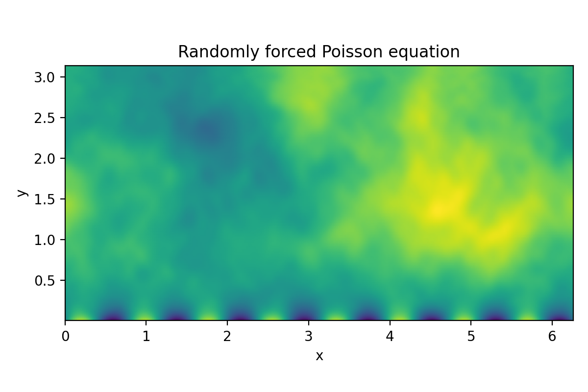
Dedalus script solving the 2D Poisson equation with mixed boundary conditions.
This script demonstrates solving a 2D Cartesian linear boundary value problem
and produces a plot of the solution. It should take just a few seconds to run.

We use a Fourier(x) * Chebyshev(y) discretization to solve the LBVP:
    dx(dx(u)) + dy(dy(u)) = f
    u(y=0) = g
    dy(u)(y=Ly) = h

For a scalar Laplacian on a finite interval, we need two tau terms. Here we
choose to lift them to the natural output (second derivative) basis.

To run and plot:
    $ python3 poisson.py
"""

import numpy as np
import matplotlib.pyplot as plt
import dedalus.public as d3
import logging
logger = logging.getLogger(__name__)


# Parameters
Lx, Ly = 2*np.pi, np.pi
Nx, Ny = 256, 128
dtype = np.float64

# Bases
coords = d3.CartesianCoordinates('x', 'y')
dist = d3.Distributor(coords, dtype=dtype)
xbasis = d3.RealFourier(coords['x'], size=Nx, bounds=(0, Lx))
ybasis = d3.Chebyshev(coords['y'], size=Ny, bounds=(0, Ly))

# Fields
u = dist.Field(name='u', bases=(xbasis, ybasis))
tau_1 = dist.Field(name='tau_1', bases=xbasis)
tau_2 = dist.Field(name='tau_2', bases=xbasis)

# Forcing
x, y = dist.local_grids(xbasis, ybasis)
f = dist.Field(bases=(xbasis, ybasis))
g = dist.Field(bases=xbasis)
h = dist.Field(bases=xbasis)
f.fill_random('g', seed=40)
f.low_pass_filter(shape=(64, 32))
g['g'] = np.sin(8*x) * 0.025
h['g'] = 0

# Substitutions
dy = lambda A: d3.Differentiate(A, coords['y'])
lift_basis = ybasis.derivative_basis(2)
lift = lambda A, n: d3.Lift(A, lift_basis, n)

# Problem
problem = d3.LBVP([u, tau_1, tau_2], namespace=locals())
problem.add_equation("lap(u) + lift(tau_1,-1) + lift(tau_2,-2) = f")
problem.add_equation("u(y=0) = g")
problem.add_equation("dy(u)(y=Ly) = h")

# Solver
solver = problem.build_solver()
solver.solve()

# Gather global data
x = xbasis.global_grid()
y = ybasis.global_grid()
ug = u.allgather_data('g')

# Plot
if dist.comm.rank == 0:
    plt.figure(figsize=(6, 4))
    plt.pcolormesh(x.ravel(), y.ravel(), ug.T, cmap='viridis', shading='gouraud', rasterized=True)
    plt.gca().set_aspect('equal')
    plt.xlabel('x')
    plt.ylabel('y')
    plt.title("Randomly forced Poisson equation")
    plt.tight_layout()
    plt.savefig('poisson.pdf')
    plt.savefig('poisson.png', dpi=200)

Output