"""
Dedalus script simulating the viscous shallow water equations on a sphere. This
script demonstrates solving an initial value problem on the sphere. It can be
ran serially or in parallel, and uses the built-in analysis framework to save
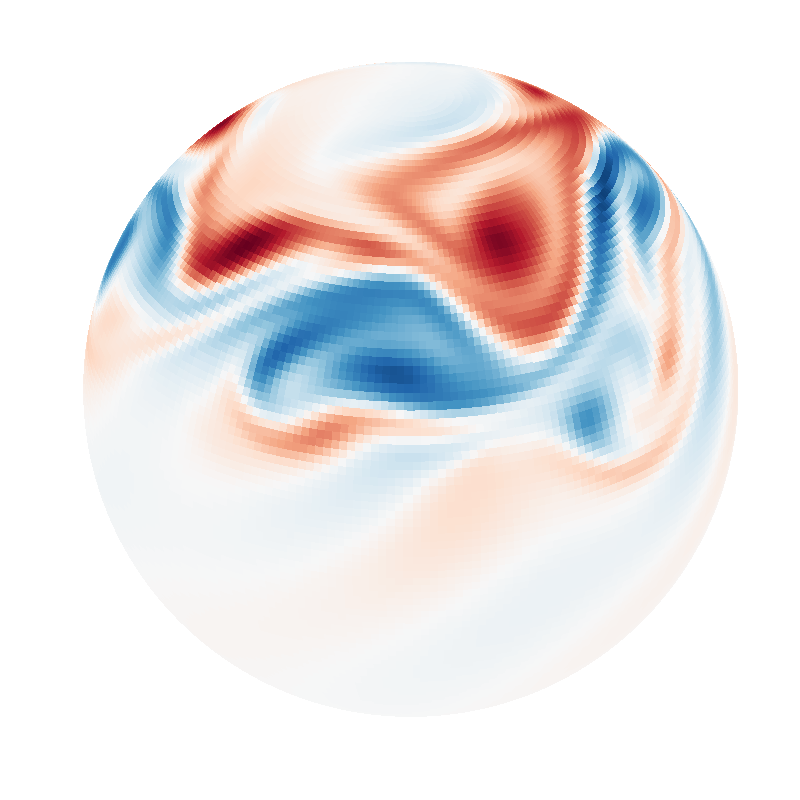
data snapshots to HDF5 files. The `plot_sphere.py` script can be used to produce
plots from the saved data. The simulation should about 5 cpu-minutes to run.
The script implements the test case of a barotropically unstable mid-latitude
jet from Galewsky et al. 2004 (https://doi.org/10.3402/tellusa.v56i5.14436).
The initial height field balanced the imposed jet is solved with an LBVP.
A perturbation is then added and the solution is evolved as an IVP.
To run and plot using e.g. 4 processes:
$ mpiexec -n 4 python3 shallow_water.py
$ mpiexec -n 4 python3 plot_sphere.py snapshots/*.h5
"""
import numpy as np
import dedalus.public as d3
import logging
logger = logging.getLogger(__name__)
# Simulation units
meter = 1 / 6.37122e6
hour = 1
second = hour / 3600
# Parameters
Nphi = 256
Ntheta = 128
dealias = 3/2
R = 6.37122e6 * meter
Omega = 7.292e-5 / second
nu = 1e5 * meter**2 / second / 32**2 # Hyperdiffusion matched at ell=32
g = 9.80616 * meter / second**2
H = 1e4 * meter
timestep = 600 * second
stop_sim_time = 360 * hour
dtype = np.float64
# Bases
coords = d3.S2Coordinates('phi', 'theta')
dist = d3.Distributor(coords, dtype=dtype)
basis = d3.SphereBasis(coords, (Nphi, Ntheta), radius=R, dealias=dealias, dtype=dtype)
# Fields
u = dist.VectorField(coords, name='u', bases=basis)
h = dist.Field(name='h', bases=basis)
# Substitutions
zcross = lambda A: d3.MulCosine(d3.skew(A))
# Initial conditions: zonal jet
phi, theta = dist.local_grids(basis)
lat = np.pi / 2 - theta + 0*phi
umax = 80 * meter / second
lat0 = np.pi / 7
lat1 = np.pi / 2 - lat0
en = np.exp(-4 / (lat1 - lat0)**2)
jet = (lat0 <= lat) * (lat <= lat1)
u_jet = umax / en * np.exp(1 / (lat[jet] - lat0) / (lat[jet] - lat1))
u['g'][0][jet] = u_jet
# Initial conditions: balanced height
c = dist.Field(name='c')
problem = d3.LBVP([h, c], namespace=locals())
problem.add_equation("g*lap(h) + c = - div(u@grad(u) + 2*Omega*zcross(u))")
problem.add_equation("ave(h) = 0")
solver = problem.build_solver()
solver.solve()
# Initial conditions: perturbation
lat2 = np.pi / 4
hpert = 120 * meter
alpha = 1 / 3
beta = 1 / 15
h['g'] += hpert * np.cos(lat) * np.exp(-(phi/alpha)**2) * np.exp(-((lat2-lat)/beta)**2)
# Problem
problem = d3.IVP([u, h], namespace=locals())
problem.add_equation("dt(u) + nu*lap(lap(u)) + g*grad(h) + 2*Omega*zcross(u) = - u@grad(u)")
problem.add_equation("dt(h) + nu*lap(lap(h)) + H*div(u) = - div(h*u)")
# Solver
solver = problem.build_solver(d3.RK222)
solver.stop_sim_time = stop_sim_time
# Analysis
snapshots = solver.evaluator.add_file_handler('snapshots', sim_dt=1*hour, max_writes=10)
snapshots.add_task(h, name='height')
snapshots.add_task(-d3.div(d3.skew(u)), name='vorticity')
# Main loop
try:
logger.info('Starting main loop')
while solver.proceed:
solver.step(timestep)
if (solver.iteration-1) % 10 == 0:
logger.info('Iteration=%i, Time=%e, dt=%e' %(solver.iteration, solver.sim_time, timestep))
except:
logger.error('Exception raised, triggering end of main loop.')
raise
finally:
solver.log_stats()