"""
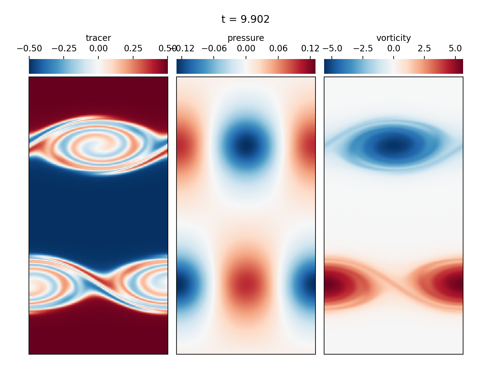
Dedalus script simulating a 2D periodic incompressible shear flow with a passive
tracer field for visualization. This script demonstrates solving a 2D periodic
initial value problem. It can be ran serially or in parallel, and uses the
built-in analysis framework to save data snapshots to HDF5 files. The
`plot_snapshots.py` script can be used to produce plots from the saved data.
The simulation should take about 10 cpu-minutes to run.
The initial flow is in the x-direction and depends only on z. The problem is
non-dimensionalized usign the shear-layer spacing and velocity jump, so the
resulting viscosity and tracer diffusivity are related to the Reynolds and
Schmidt numbers as:
nu = 1 / Reynolds
D = nu / Schmidt
To run and plot using e.g. 4 processes:
$ mpiexec -n 4 python3 shear_flow.py
$ mpiexec -n 4 python3 plot_snapshots.py snapshots/*.h5
"""
import numpy as np
import dedalus.public as d3
import logging
logger = logging.getLogger(__name__)
# Parameters
Lx, Lz = 1, 2
Nx, Nz = 128, 256
Reynolds = 5e4
Schmidt = 1
dealias = 3/2
stop_sim_time = 20
timestepper = d3.RK222
max_timestep = 1e-2
dtype = np.float64
# Bases
coords = d3.CartesianCoordinates('x', 'z')
dist = d3.Distributor(coords, dtype=dtype)
xbasis = d3.RealFourier(coords['x'], size=Nx, bounds=(0, Lx), dealias=dealias)
zbasis = d3.RealFourier(coords['z'], size=Nz, bounds=(-Lz/2, Lz/2), dealias=dealias)
# Fields
p = dist.Field(name='p', bases=(xbasis,zbasis))
s = dist.Field(name='s', bases=(xbasis,zbasis))
u = dist.VectorField(coords, name='u', bases=(xbasis,zbasis))
tau_p = dist.Field(name='tau_p')
# Substitutions
nu = 1 / Reynolds
D = nu / Schmidt
x, z = dist.local_grids(xbasis, zbasis)
ex, ez = coords.unit_vector_fields(dist)
# Problem
problem = d3.IVP([u, s, p, tau_p], namespace=locals())
problem.add_equation("dt(u) + grad(p) - nu*lap(u) = - u@grad(u)")
problem.add_equation("dt(s) - D*lap(s) = - u@grad(s)")
problem.add_equation("div(u) + tau_p = 0")
problem.add_equation("integ(p) = 0") # Pressure gauge
# Solver
solver = problem.build_solver(timestepper)
solver.stop_sim_time = stop_sim_time
# Initial conditions
# Background shear
u['g'][0] = 1/2 + 1/2 * (np.tanh((z-0.5)/0.1) - np.tanh((z+0.5)/0.1))
# Match tracer to shear
s['g'] = u['g'][0]
# Add small vertical velocity perturbations localized to the shear layers
u['g'][1] += 0.1 * np.sin(2*np.pi*x/Lx) * np.exp(-(z-0.5)**2/0.01)
u['g'][1] += 0.1 * np.sin(2*np.pi*x/Lx) * np.exp(-(z+0.5)**2/0.01)
# Analysis
snapshots = solver.evaluator.add_file_handler('snapshots', sim_dt=0.1, max_writes=10)
snapshots.add_task(s, name='tracer')
snapshots.add_task(p, name='pressure')
snapshots.add_task(-d3.div(d3.skew(u)), name='vorticity')
# CFL
CFL = d3.CFL(solver, initial_dt=max_timestep, cadence=10, safety=0.2, threshold=0.1,
max_change=1.5, min_change=0.5, max_dt=max_timestep)
CFL.add_velocity(u)
# Flow properties
flow = d3.GlobalFlowProperty(solver, cadence=10)
flow.add_property((u@ez)**2, name='w2')
# Main loop
try:
logger.info('Starting main loop')
while solver.proceed:
timestep = CFL.compute_timestep()
solver.step(timestep)
if (solver.iteration-1) % 10 == 0:
max_w = np.sqrt(flow.max('w2'))
logger.info('Iteration=%i, Time=%e, dt=%e, max(w)=%f' %(solver.iteration, solver.sim_time, timestep, max_w))
except:
logger.error('Exception raised, triggering end of main loop.')
raise
finally:
solver.log_stats()