Axisymmetric Taylor-Couette flow in Dedalus

(image: wikipedia)

Taylor-Couette flow is characterized by three dimensionless numbers:

\(\eta = R1/R2\), the ratio of the inner cylidner radius \(R_1\) to the outer cylinder radius \(R_2\)

\(\mu = \Omega_2/\Omega_1\), the ratio of the OUTER cylinder rotation rate \(\Omega_2\) to the inner rate \(\Omega_1\)

\(\mathrm{Re} = \Omega_1 R_1 \delta/\nu\), the Reynolds numbers, where \(\delta = R_2 - R_1\), the gap width between the cylinders

We non dimensionalize the flow in terms of

\([\mathrm{L}] = \delta = R_2 - R_1\)

\([\mathrm{V}] = R_1 \Omega_1\)

\([\mathrm{M}] = \rho \delta^3\)

And choose \(\delta = 1\), \(R_1 \Omega_1 = 1\), and \(\rho = 1\).

%pylab inline

%pylab is deprecated, use %matplotlib inline and import the required libraries.
Populating the interactive namespace from numpy and matplotlib

import numpy as np
import time
import h5py

import dedalus.public as de
from dedalus.extras import flow_tools

import logging
logger = logging.getLogger(__name__)

Input parameters

These parameters are taken from Barenghi (1991) J. Comp. Phys. We’ll compute the growth rate and compare it to the value \(\gamma_{analytic} = 0.430108693\)

# Input parameters from Barenghi (1991)
eta = 1./1.444 # R1/R2
alpha = 3.13   # vertical wavenumber
Re = 80.       # in units of R1*Omega1*delta/nu
mu = 0.        # Omega2/Omega1

# Computed quantitites
omega_in = 1.
omega_out = mu * omega_in
r_in = eta/(1. - eta)
r_out = 1./(1. - eta)
height = 2.*np.pi/alpha
v_l = 1. # by default, we set v_l to 1.
v_r = omega_out*r_out

Problem Domain

Every PDE takes place somewhere, so we define a domain, which in this case is the \(z\) and \(r\) directions. Because the \(r\) direction has walls, we use a Chebyshev basis, but the \(z\) direction is periodic, so we use a Fourier basis. The Domain object combines these.

# Create bases
r_basis = de.Chebyshev('r', 32, interval=(r_in, r_out), dealias=3/2)
z_basis = de.Fourier('z', 32, interval=(0., height), dealias=3/2)
domain = de.Domain([z_basis, r_basis], grid_dtype=np.float64)

Equations

We use the IVP object, which can parse a set of equations in plain text and combine them into an initial value problem.

Here, we code up the equations for the “primative” variables, \(\mathbf{v} = u \mathbf{\hat{r}} + v \mathbf{\hat{\theta}} + w \mathbf{\hat{z}}\) and \(p\), along with their first derivatives.

The equations are the incompressible, axisymmetric Navier-Stokes equations in cylindrical coordinates

The axes will be called \(z\) and \(r\), and we will expand the non-constant \(r^2\) terms, to a cutoff precision of \(10^{-8}\). These non-constant coefficients (called “NCC” in Dedalus) are geometric here, but they could be background states in convection, position dependent diffusion coefficients, etc.

We also add the parameters to the object, so we can use their names in the equations below.

TC = de.IVP(domain, variables=['p', 'u', 'v', 'w', 'ur', 'vr', 'wr'], ncc_cutoff=1e-8)
TC.parameters['nu'] = 1./Re
TC.parameters['v_l'] = v_l
TC.parameters['v_r'] = v_r
mu = TC.parameters['v_r']/TC.parameters['v_l'] * eta

The equations are multiplied through by \(r^2\), so that there are no \(1/r\) terms, which require more coefficients in the expansion.

TC.add_equation("r*ur + u + r*dz(w) = 0")
TC.add_equation("r*r*dt(u) - r*r*nu*dr(ur) - r*nu*ur - r*r*nu*dz(dz(u)) + nu*u + r*r*dr(p) = -r*r*u*ur - r*r*w*dz(u) + r*v*v")
TC.add_equation("r*r*dt(v) - r*r*nu*dr(vr) - r*nu*vr - r*r*nu*dz(dz(v)) + nu*v  = -r*r*u*vr - r*r*w*dz(v) - r*u*v")
TC.add_equation("r*dt(w) - r*nu*dr(wr) - nu*wr - r*nu*dz(dz(w)) + r*dz(p) = -r*u*wr - r*w*dz(w)")
TC.add_equation("ur - dr(u) = 0")
TC.add_equation("vr - dr(v) = 0")
TC.add_equation("wr - dr(w) = 0")

Initial and Boundary Conditions

First we create some aliases to the \(r\) and \(z\) grids, so we can quickly compute the analytic Couette flow solution for unperturbed, unstable axisymmetric flow.

r = domain.grid(1, scales=domain.dealias)
z = domain.grid(0, scales=domain.dealias)

p_analytic = (eta/(1-eta**2))**2 * (-1./(2*r**2*(1-eta)**2) -2*np.log(r) +0.5*r**2 * (1.-eta)**2)
v_analytic = eta/(1-eta**2) * ((1. - mu)/(r*(1-eta)) - r * (1.-eta) * (1 - mu/eta**2))

And now we add boundary conditions, simply by typing them in plain text, just like the equations.

# boundary conditions
TC.add_bc("left(u) = 0")
TC.add_bc("left(v) = v_l")
TC.add_bc("left(w) = 0")
TC.add_bc("right(u) = 0", condition="nz != 0")
TC.add_bc("right(v) = v_r")
TC.add_bc("right(w) = 0")
TC.add_bc("left(p) = 0", condition="nz == 0")

We can now set the parameters of the problem, \(\nu\), \(v_l\), and \(v_r\), and have the code log \(\mu\) to the output (which can be stdout, a file, or both).

Timestepping

We have implemented a variety of multi-step and Runge-Kutta implicit-explicit timesteppers in Dedalus. The available options can be seen in the timesteppers.py module. Here we pick RK443, an IMEX Runga-Kutta scheme. We set our maximum timestep max_dt, and choose the various stopping parameters.

Finally, we’ve got our full initial value problem (represented by the IVP) object: a timestepper, a domain, and a ParsedProblem (or equation set).

dt = max_dt = 1.
omega1 = TC.parameters['v_l']/r_in
period = 2*np.pi/omega1

ts = de.timesteppers.RK443
IVP = TC.build_solver(ts)
IVP.stop_sim_time = 15.*period
IVP.stop_wall_time = np.inf
IVP.stop_iteration = 10000000

2022-08-26 11:21:12,977 pencil 0/1 INFO :: Building pencil matrix 1/16 (~6%) Elapsed: 0s, Remaining: 0s, Rate: 4.5e+01/s
2022-08-26 11:21:12,991 pencil 0/1 INFO :: Building pencil matrix 2/16 (~12%) Elapsed: 0s, Remaining: 0s, Rate: 5.5e+01/s
2022-08-26 11:21:13,018 pencil 0/1 INFO :: Building pencil matrix 4/16 (~25%) Elapsed: 0s, Remaining: 0s, Rate: 6.3e+01/s
2022-08-26 11:21:13,049 pencil 0/1 INFO :: Building pencil matrix 6/16 (~38%) Elapsed: 0s, Remaining: 0s, Rate: 6.4e+01/s
2022-08-26 11:21:13,078 pencil 0/1 INFO :: Building pencil matrix 8/16 (~50%) Elapsed: 0s, Remaining: 0s, Rate: 6.5e+01/s
2022-08-26 11:21:13,106 pencil 0/1 INFO :: Building pencil matrix 10/16 (~62%) Elapsed: 0s, Remaining: 0s, Rate: 6.6e+01/s
2022-08-26 11:21:13,134 pencil 0/1 INFO :: Building pencil matrix 12/16 (~75%) Elapsed: 0s, Remaining: 0s, Rate: 6.7e+01/s
2022-08-26 11:21:13,161 pencil 0/1 INFO :: Building pencil matrix 14/16 (~88%) Elapsed: 0s, Remaining: 0s, Rate: 6.8e+01/s
2022-08-26 11:21:13,190 pencil 0/1 INFO :: Building pencil matrix 16/16 (~100%) Elapsed: 0s, Remaining: 0s, Rate: 6.8e+01/s

We initialize the state vector, given by IVP.state. To make life a little easier, we set some aliases first:

p = IVP.state['p']
u = IVP.state['u']
v = IVP.state['v']
w = IVP.state['w']
ur = IVP.state['ur']
vr = IVP.state['vr']
wr = IVP.state['wr']

Next, we create a new field, \(\phi\), defined on the domain, which we’ll use below to compute incompressible, random velocity perturbations.

phi = domain.new_field(name='phi')

Here, we set all the fields and states to their dealiased domains. Dedalus allows us to set the “scale” of our data: this allows us to interpolate our data to a grid of any size at spectral accuracy. Of course, this isn’t CSI: Fluid Dynamics, so you won’t get any more detail than your highest spectral coefficient.

for f in [phi,p,u,v,w,ur,vr,wr]:
    f.set_scales(domain.dealias, keep_data=False)

Now we set the state vector with our previously computed analytic solution and compute the first derivatives (to make our system first order).

v['g'] = v_analytic
# p['g'] = p_analytic

v.differentiate('r',out=vr)

<Field 5196112960>

And finally, we set some small, incompressible perturbations to the velocity field so we can kick off our linear instability.

First, we initialize \(\phi\) (which we created above) to Gaussian noise and then mask it to only appear in the center of the domain, so we don’t violate the boundary conditions. We then take its curl to get the velocity perturbations.

Unfortunately, Gaussian noise on the grid is generally a bad idea: zone-to-zone variations (that is, the highest frequency components) will be amplified arbitrarily by any differentiation. So, let’s filter out those high frequency components using this handy little function:

def filter_field(field,frac=0.5):
    dom = field.domain
    local_slice = dom.dist.coeff_layout.slices(scales=dom.dealias)
    coeff = []
    for i in range(dom.dim)[::-1]:
        coeff.append(np.linspace(0,1,dom.global_coeff_shape[i],endpoint=False))
    cc = np.meshgrid(*coeff)

    field_filter = np.zeros(dom.local_coeff_shape,dtype='bool')
    for i in range(dom.dim):
        field_filter = field_filter | (cc[i][local_slice] > frac)
    field['c'][field_filter] = 0j

This is not the best filter: it assumes that cutting off above a certain Chebyshev mode \(n\) and Fourier mode \(n\) will be OK, though this may produce anisotropies in the data (I haven’t checked). If you’re worrying about the anisotropy of the initial noise of your ICs, you can always replace this filter with something better.

# incompressible perturbation, arbitrary vorticity
# u = -dz(phi)
# w = dr(phi) + phi/r

phi['g'] = 1e-3* np.random.randn(*v['g'].shape)*np.sin(np.pi*(r - r_in))
filter_field(phi)
phi.differentiate('z',out=u)
u['g'] *= -1
phi.differentiate('r',out=w)
w['g'] += phi['g']/r

u.differentiate('r',out=ur)
w.differentiate('r',out=wr)

<Field 5196112912>

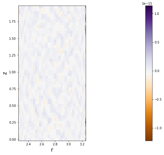
Now we check that incompressibility is indeed satisfied, first by computing \(\nabla \cdot u\),

divu0 = domain.new_field(name='divu0')
u.differentiate('r',out=divu0)
divu0['g'] += u['g']/r + w.differentiate('z')['g']

and then by plotting it to make sure it’s nowhere greater than \(\sim 10^{-15}\).

figsize(12,8)
pcolormesh((r[0]*ones_like(z)).T,(z*ones_like(r)).T,divu0['g'].T,cmap='PuOr')
colorbar()
axis('image')
xlabel('r', fontsize=18)
ylabel('z', fontsize=18)

Text(0, 0.5, 'z')

Time step size and the CFL condition

Here, we use the nice CFL calculator provided by the flow_tools package in the extras module.

CFL = flow_tools.CFL(IVP, initial_dt=1e-3, cadence=5, safety=0.3,
                     max_change=1.5, min_change=0.5)
CFL.add_velocities(('u', 'w'))

Analysis

Dedalus has a very powerful inline analysis system, and here we set up a few.

# Integrated energy every 10 iterations.
analysis1 = IVP.evaluator.add_file_handler("scalar_data", iter=10)
analysis1.add_task("integ(0.5 * (u*u + v*v + w*w))", name="total kinetic energy")
analysis1.add_task("integ(0.5 * (u*u + w*w))", name="meridional kinetic energy")
analysis1.add_task("integ((u*u)**0.5)", name='u_rms')
analysis1.add_task("integ((w*w)**0.5)", name='w_rms')

# Snapshots every half an inner rotation period.
analysis2 = IVP.evaluator.add_file_handler('snapshots',sim_dt=0.5*period, max_size=2**30)
analysis2.add_system(IVP.state, layout='g')

# Radial profiles every 100 timesteps.
analysis3 = IVP.evaluator.add_file_handler("radial_profiles", iter=100)
analysis3.add_task("integ(r*v, 'z')", name='Angular Momentum')

The Main Loop

And here we actually run the simulation!

dt = CFL.compute_dt()
# Main loop
start_time = time.time()

while IVP.ok:
    IVP.step(dt)
    if IVP.iteration % 10 == 0:
        logger.info('Iteration: %i, Time: %e, dt: %e' %(IVP.iteration, IVP.sim_time, dt))
    dt = CFL.compute_dt()


end_time = time.time()

# Print statistics
logger.info('Total time: %f' %(end_time-start_time))
logger.info('Iterations: %i' %IVP.iteration)
logger.info('Average timestep: %f' %(IVP.sim_time/IVP.iteration))

2022-08-26 11:21:14,422 __main__ 0/1 INFO :: Iteration: 10, Time: 1.200000e-02, dt: 1.500000e-03
2022-08-26 11:21:14,644 __main__ 0/1 INFO :: Iteration: 20, Time: 3.825000e-02, dt: 3.375000e-03
2022-08-26 11:21:14,870 __main__ 0/1 INFO :: Iteration: 30, Time: 9.731250e-02, dt: 7.593750e-03
2022-08-26 11:21:15,096 __main__ 0/1 INFO :: Iteration: 40, Time: 2.302031e-01, dt: 1.708594e-02
2022-08-26 11:21:15,346 __main__ 0/1 INFO :: Iteration: 50, Time: 5.292070e-01, dt: 3.844336e-02
2022-08-26 11:21:15,582 __main__ 0/1 INFO :: Iteration: 60, Time: 1.201966e+00, dt: 8.649756e-02
2022-08-26 11:21:15,806 __main__ 0/1 INFO :: Iteration: 70, Time: 2.715673e+00, dt: 1.946195e-01
2022-08-26 11:21:16,031 __main__ 0/1 INFO :: Iteration: 80, Time: 6.121514e+00, dt: 4.378939e-01
2022-08-26 11:21:16,271 __main__ 0/1 INFO :: Iteration: 90, Time: 1.378466e+01, dt: 9.852613e-01
2022-08-26 11:21:16,549 __main__ 0/1 INFO :: Iteration: 100, Time: 3.102673e+01, dt: 2.216838e+00
2022-08-26 11:21:16,877 __main__ 0/1 INFO :: Iteration: 110, Time: 6.982139e+01, dt: 4.987885e+00
2022-08-26 11:21:17,223 __main__ 0/1 INFO :: Iteration: 120, Time: 1.571094e+02, dt: 1.122274e+01
2022-08-26 11:21:17,399 solvers 0/1 INFO :: Simulation stop time reached.
2022-08-26 11:21:17,400 __main__ 0/1 INFO :: Total time: 3.403150
2022-08-26 11:21:17,400 __main__ 0/1 INFO :: Iterations: 124
2022-08-26 11:21:17,401 __main__ 0/1 INFO :: Average timestep: 1.764794

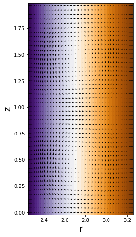
Analysis

First, let’s look at our last time snapshot, plotting the background \(v \mathbf{\hat{\theta}}\) velocity with arrows representing the meridional flow:

figsize(12,8)
pcolormesh((r[0]*ones_like(z)).T,(z*ones_like(r)).T,v['g'].T,cmap='PuOr')
quiver((r[0]*ones_like(z)).T,(z*ones_like(r)).T,u['g'].T,w['g'].T,width=0.005)
axis('image')
xlabel('r', fontsize=18)
ylabel('z', fontsize=18)

Text(0, 0.5, 'z')

But we really want some quantitative comparison with the growth rate \(\gamma_{analytic}\) from Barenghi (1991). First we construct a small helper function to read our timeseries data, and then we load it out of the self-documented HDF5 file.

def get_timeseries(data, field):
    data_1d = []
    time = data['scales/sim_time'][:]
    data_out = data['tasks/%s'%field][:,0,0]
    return time, data_out

data = h5py.File("scalar_data/scalar_data_s1/scalar_data_s1_p0.h5", "r")
t, ke = get_timeseries(data, 'total kinetic energy')
t, kem = get_timeseries(data, 'meridional kinetic energy')
t, urms = get_timeseries(data, 'u_rms')
t, wrms = get_timeseries(data, 'w_rms')

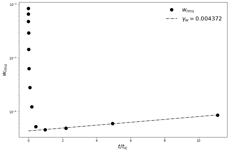
In order to compare to Barenghi (1991), we scale our results by the Reynolds number, because we have non-dimensionalized slightly differently than he did.

t_window = (t/period > 2) & (t/period < 14)

gamma_w, log_w0 = np.polyfit(t[t_window], np.log(wrms[t_window]),1)

gamma_w_scaled = gamma_w*Re
gamma_barenghi = 0.430108693
rel_error_barenghi = (gamma_barenghi - gamma_w_scaled)/gamma_barenghi

print("gamma_w = %10.8f" % gamma_w_scaled)
print("relative error = %10.8e" % rel_error_barenghi)

gamma_w = 0.34977333
relative error = 1.86779212e-01

This looks like a rather high error (order 10% or so), but we know from Barenghi (1991) that the error is dominated by the timestep. Here, we’ve used a very loose timestep, but if you fix \(dt\) (rather than using the CFL calculator), you can get much lower errors at the cost of a longer run.

Finally, we plot the RMS \(w\) velocity, and compare it with the fitted exponential solution

fig = figure()
ax = fig.add_subplot(111)
ax.semilogy(t/period, wrms, 'ko', label=r'$w_{rms}$',ms=10)
ax.semilogy(t/period, np.exp(log_w0)*np.exp(gamma_w*t), 'k-.', label='$\gamma_w = %f$' % gamma_w)
ax.legend(loc='upper right',fontsize=18).draw_frame(False)
ax.set_xlabel(r"$t/t_{ic}$",fontsize=18)
ax.set_ylabel(r"$w_{rms}$",fontsize=18)

fig.savefig('growth_rates.png')