Kelvin-Helmholtz Instability

(image: Chuck Doswell)

We will simulate the incompressible Kelvin-Helmholtz problem. We non-dimensionalize the problem by taking the box height to be one and the jump in velocity to be one. Then the Reynolds number is given by

\[\mathrm{Re} = \frac{U H}{\nu} = \frac{1}{\nu}.\]

We use no slip boundary conditions, and a box with aspect ratio \(L/H=2\). The initial velocity profile is given by a hyperbolic tangent, and only a single mode is initially excited. We will also track a passive scalar which will help us visualize the instability.

First, we import the necessary modules.

%matplotlib inline

import numpy as np
import matplotlib.pyplot as plt
import h5py
import time
from IPython import display

from dedalus import public as de
from dedalus.extras import flow_tools

import logging
logger = logging.getLogger(__name__)

To perform an initial value problem (IVP) in Dedalus, you need three things:

1. A domain to solve the problem on

2. Equations to solve

3. A timestepping scheme

Problem Domain

First, we will specify the domain. Domains are built by taking the direct product of bases. Here we are running a 2D simulation, so we will define \(x\) and \(y\) bases. From these, we build the domain.

# Aspect ratio 2
Lx, Ly = (2., 1.)
nx, ny = (192, 96)

# Create bases and domain
x_basis = de.Fourier('x', nx, interval=(0, Lx), dealias=3/2)
y_basis = de.Chebyshev('y',ny, interval=(-Ly/2, Ly/2), dealias=3/2)
domain = de.Domain([x_basis, y_basis], grid_dtype=np.float64)

The last basis (\(y\) direction) is represented in Chebyshev polynomials. This will allow us to apply interesting boundary conditions in the \(y\) direction. We call the other directions (in this case just \(x\)) the “horizontal” directions. The horizontal directions must be “easy” in the sense that taking derivatives cannot couple different horizontal modes. Right now, we have Fourier and Sin/Cos series implemented for the horizontal directions, and are working on implementing spherical harmonics.

Equations

Next we will define the equations that will be solved on this domain. The equations are

\[\partial_t u + \boldsymbol{u}\boldsymbol{\cdot}\boldsymbol{\nabla} u + \partial_x p = \frac{1}{{\rm Re}} \nabla^2 u\]

\[\partial_t v + \boldsymbol{u}\boldsymbol{\cdot}\boldsymbol{\nabla} v + \partial_y p = \frac{1}{{\rm Re}} \nabla^2 v\]

\[\boldsymbol{\nabla}\boldsymbol{\cdot}\boldsymbol{u} = 0\]

\[\partial_t s + \boldsymbol{u}\boldsymbol{\cdot}\boldsymbol{\nabla} s = \frac{1}{{\rm Re}{\rm Sc}} \nabla^2 s\]

The equations are written such that the left-hand side (LHS) is treated implicitly, and the right-hand side (RHS) is treated explicitly. The LHS is limited to only linear terms, though linear terms can also be placed on the RHS. Since \(y\) is our special direction in this example, we also restrict the LHS to be at most first order in derivatives with respect to \(y\).

We also set the parameters, the Reynolds and Schmidt numbers.

Reynolds = 1e4
Schmidt = 1.

problem = de.IVP(domain, variables=['p','u','v','uy','vy','S','Sy'])
problem.parameters['Re'] = Reynolds
problem.parameters['Sc'] = Schmidt
problem.add_equation("dt(u) + dx(p) - 1/Re*(dx(dx(u)) + dy(uy)) = - u*dx(u) - v*uy")
problem.add_equation("dt(v) + dy(p) - 1/Re*(dx(dx(v)) + dy(vy)) = - u*dx(v) - v*vy")
problem.add_equation("dx(u) + vy = 0")
problem.add_equation("dt(S) - 1/(Re*Sc)*(dx(dx(S)) + dy(Sy)) = - u*dx(S) - v*Sy")
problem.add_equation("uy - dy(u) = 0")
problem.add_equation("vy - dy(v) = 0")
problem.add_equation("Sy - dy(S) = 0")

Because we are using this first-order formalism, we define auxiliary variables uy, vy, and Sy to be the \(y\)-derivative of u, v, and S respectively.

Next, we set our boundary conditions. “Left” boundary conditions are applied at \(y=-Ly/2\) and “right” boundary conditions are applied at \(y=+Ly/2\).

problem.add_bc("left(u) = 0.5")
problem.add_bc("right(u) = -0.5")
problem.add_bc("left(v) = 0")
problem.add_bc("right(v) = 0", condition="(nx != 0)")
problem.add_bc("left(p) = 0", condition="(nx == 0)")
problem.add_bc("left(S) = 0")
problem.add_bc("right(S) = 1")

Note that we have a special boundary condition for the \(k_x=0\) mode (singled out by condition="(nx==0)"). This is because the continuity equation implies \(\partial_y v=0\) if \(k_x=0\); thus, \(v=0\) on the top and bottom are redundant boundary conditions. We replace one of these with a gauge choice for the pressure.

Timestepping

We have implemented a variety of multi-step and Runge-Kutta implicit-explicit timesteppers in Dedalus. The available options can be seen in the timesteppers.py module. For this problem, we will use a third-order, four-stage Runge-Kutta integrator. Changing the timestepping algorithm is as easy as changing one line of code.

ts = de.timesteppers.RK443

Initial Value Problem

We now have the three ingredients necessary to set up our IVP:

solver =  problem.build_solver(ts)

2022-08-26 11:24:29,478 pencil 0/1 INFO :: Building pencil matrix 1/96 (~1%) Elapsed: 0s, Remaining: 1s, Rate: 7.3e+01/s
2022-08-26 11:24:29,590 pencil 0/1 INFO :: Building pencil matrix 10/96 (~10%) Elapsed: 0s, Remaining: 1s, Rate: 8.0e+01/s
2022-08-26 11:24:29,711 pencil 0/1 INFO :: Building pencil matrix 20/96 (~21%) Elapsed: 0s, Remaining: 1s, Rate: 8.1e+01/s
2022-08-26 11:24:29,833 pencil 0/1 INFO :: Building pencil matrix 30/96 (~31%) Elapsed: 0s, Remaining: 1s, Rate: 8.1e+01/s
2022-08-26 11:24:29,963 pencil 0/1 INFO :: Building pencil matrix 40/96 (~42%) Elapsed: 0s, Remaining: 1s, Rate: 8.0e+01/s
2022-08-26 11:24:30,090 pencil 0/1 INFO :: Building pencil matrix 50/96 (~52%) Elapsed: 1s, Remaining: 1s, Rate: 8.0e+01/s
2022-08-26 11:24:30,211 pencil 0/1 INFO :: Building pencil matrix 60/96 (~62%) Elapsed: 1s, Remaining: 0s, Rate: 8.0e+01/s
2022-08-26 11:24:30,335 pencil 0/1 INFO :: Building pencil matrix 70/96 (~73%) Elapsed: 1s, Remaining: 0s, Rate: 8.0e+01/s
2022-08-26 11:24:30,474 pencil 0/1 INFO :: Building pencil matrix 80/96 (~83%) Elapsed: 1s, Remaining: 0s, Rate: 7.9e+01/s
2022-08-26 11:24:30,606 pencil 0/1 INFO :: Building pencil matrix 90/96 (~94%) Elapsed: 1s, Remaining: 0s, Rate: 7.9e+01/s
2022-08-26 11:24:30,686 pencil 0/1 INFO :: Building pencil matrix 96/96 (~100%) Elapsed: 1s, Remaining: 0s, Rate: 7.9e+01/s

Now we set our initial conditions. We set the horizontal velocity and scalar field to tanh profiles, and using a single-mode initial perturbation in \(v\).

x = domain.grid(0)
y = domain.grid(1)
u = solver.state['u']
uy = solver.state['uy']
v = solver.state['v']
vy = solver.state['vy']
S = solver.state['S']
Sy = solver.state['Sy']

a = 0.05
sigma = 0.2
flow = -0.5
amp = -0.2
u['g'] = flow*np.tanh(y/a)
v['g'] = amp*np.sin(2.0*np.pi*x/Lx)*np.exp(-(y*y)/(sigma*sigma))
S['g'] = 0.5*(1+np.tanh(y/a))
u.differentiate('y',out=uy)
v.differentiate('y',out=vy)
S.differentiate('y',out=Sy)

<Field 5147257408>

Now we set integration parameters and the CFL.

solver.stop_sim_time = 2.01
solver.stop_wall_time = np.inf
solver.stop_iteration = np.inf

initial_dt = 0.2*Lx/nx
cfl = flow_tools.CFL(solver,initial_dt,safety=0.8)
cfl.add_velocities(('u','v'))

Analysis

We have a sophisticated analysis framework in which the user specifies analysis tasks as strings. Users can output full data cubes, slices, volume averages, and more. Here we will only output a few 2D slices, and a 1D profile of the horizontally averaged concentration field. Data is output in the hdf5 file format.

analysis = solver.evaluator.add_file_handler('analysis_tasks', sim_dt=0.1, max_writes=50)
analysis.add_task('S')
analysis.add_task('u')
solver.evaluator.vars['Lx'] = Lx
analysis.add_task("integ(S,'x')/Lx", name='S profile')

Main Loop

We now have everything set up for our simulation. In Dedalus, the user writes their own main loop.

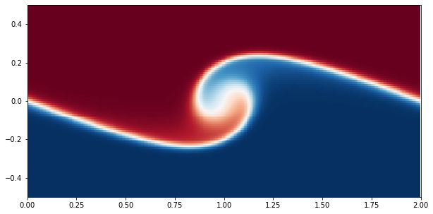
# Make plot of scalar field
x = domain.grid(0,scales=domain.dealias)
y = domain.grid(1,scales=domain.dealias)
xm, ym = np.meshgrid(x,y)
fig, axis = plt.subplots(figsize=(10,5))
p = axis.pcolormesh(xm, ym, S['g'].T, cmap='RdBu_r');
axis.set_xlim([0,2.])
axis.set_ylim([-0.5,0.5])

logger.info('Starting loop')
start_time = time.time()
while solver.ok:
    dt = cfl.compute_dt()
    solver.step(dt)
    if solver.iteration % 10 == 0:
        # Update plot of scalar field
        p.set_array(np.ravel(S['g'].T))
        display.clear_output()
        display.display(plt.gcf())
        logger.info('Iteration: %i, Time: %e, dt: %e' %(solver.iteration, solver.sim_time, dt))

end_time = time.time()

p.set_array(np.ravel(S['g'].T))
display.clear_output()
# Print statistics
logger.info('Run time: %f' %(end_time-start_time))
logger.info('Iterations: %i' %solver.iteration)

2022-08-26 11:25:50,227 __main__ 0/1 INFO :: Run time: 78.498186
2022-08-26 11:25:50,227 __main__ 0/1 INFO :: Iterations: 269

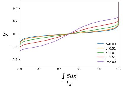
Analysis

As an example of doing some analysis, we will load in the horizontally averaged profiles of the scalar field \(s\) and plot them.

# Read in the data
f = h5py.File('analysis_tasks/analysis_tasks_s1/analysis_tasks_s1_p0.h5','r')
y = f['/scales/y/1.0'][:]
t = f['scales']['sim_time'][:]
S_ave = f['tasks']['S profile'][:]
f.close()

S_ave = S_ave[:,0,:] # remove length-one x dimension

for i in range(0,21,5):
  plt.plot(S_ave[i,:],y,label='t=%4.2f' %t[i])

plt.ylim([-0.5,0.5])
plt.xlim([0,1])
plt.xlabel(r'$\frac{\int \ S dx}{L_x}$',fontsize=24)
plt.ylabel(r'$y$',fontsize=24)
plt.legend(loc='lower right').draw_frame(False)