"""
Dedalus script solving the linear stability eigenvalue problem for pipe flow.
This script demonstrates solving an eigenvalue problem in the periodic cylinder
using the disk basis and a parametrized axial wavenumber. It should take just
a few seconds to run (serial only).
The radius of the pipe is R = 1, and the problem is non-dimensionalized using
the radius and laminar velocity, such that the background flow is w0 = 1 - r**2.
No-slip boundary conditions are implemented on the velocity perturbations.
For incompressible hydro with one boundary, we need one tau term each for the
scalar axial velocity and vector horizontal (in-disk) velocity. Here we choose
to left the tau terms to the original (k=0) basis.
The eigenvalues are compared to the results of Vasil et al. (2016) [1] in Table 3.
To run, print, and plot the slowest decaying mode:
$ python3 pipe_flow.py
References:
[1]: G. M. Vasil, K. J. Burns, D. Lecoanet, S. Olver, B. P. Brown, J. S. Oishi,
"Tensor calculus in polar coordinates using Jacobi polynomials," Journal
of Computational Physics (2016).
"""
import numpy as np
import dedalus.public as d3
import matplotlib.pyplot as plt
import logging
logger = logging.getLogger(__name__)
# Parameters
Re = 1e4
kz = 1
m = 5
Nphi = 2 * m + 2
Nr = 64
dtype = np.complex128
# Bases
coords = d3.PolarCoordinates('phi', 'r')
dist = d3.Distributor(coords, dtype=dtype)
disk = d3.DiskBasis(coords, shape=(Nphi, Nr), radius=1, dtype=dtype)
phi, r = dist.local_grids(disk)
# Fields
s = dist.Field(name='s')
u = dist.VectorField(coords, name='u', bases=disk)
w = dist.Field(name='w', bases=disk)
p = dist.Field(name='p', bases=disk)
tau_u = dist.VectorField(coords, name='tau_u', bases=disk.edge)
tau_w = dist.Field(name='tau_w', bases=disk.edge)
tau_p = dist.Field(name='tau_p')
# Substitutions
dt = lambda A: s*A
dz = lambda A: 1j*kz*A
lift_basis = disk.derivative_basis(2)
lift = lambda A: d3.Lift(A, lift_basis, -1)
# Background
w0 = dist.Field(name='w0', bases=disk.radial_basis)
w0['g'] = 1 - r**2
# Problem
problem = d3.EVP([u, w, p, tau_u, tau_w, tau_p], eigenvalue=s, namespace=locals())
problem.add_equation("div(u) + dz(w) = 0")
problem.add_equation("dt(u) + w0*dz(u) + grad(p) - (1/Re)*(lap(u)+dz(dz(u))) + lift(tau_u) = 0")
problem.add_equation("dt(w) + w0*dz(w) + u@grad(w0) + dz(p) - (1/Re)*(lap(w)+dz(dz(w))) + lift(tau_w) = 0")
problem.add_equation("u(r=1) = 0")
problem.add_equation("w(r=1) = 0")
# Solver
solver = problem.build_solver()
sp = solver.subproblems_by_group[(m, None)]
solver.solve_dense(sp)
evals = solver.eigenvalues[np.isfinite(solver.eigenvalues)]
evals = evals[np.argsort(-evals.real)]
print(f"Slowest decaying mode: λ = {evals[0]}")
solver.set_state(np.argmin(np.abs(solver.eigenvalues - evals[0])), sp.subsystems[0])
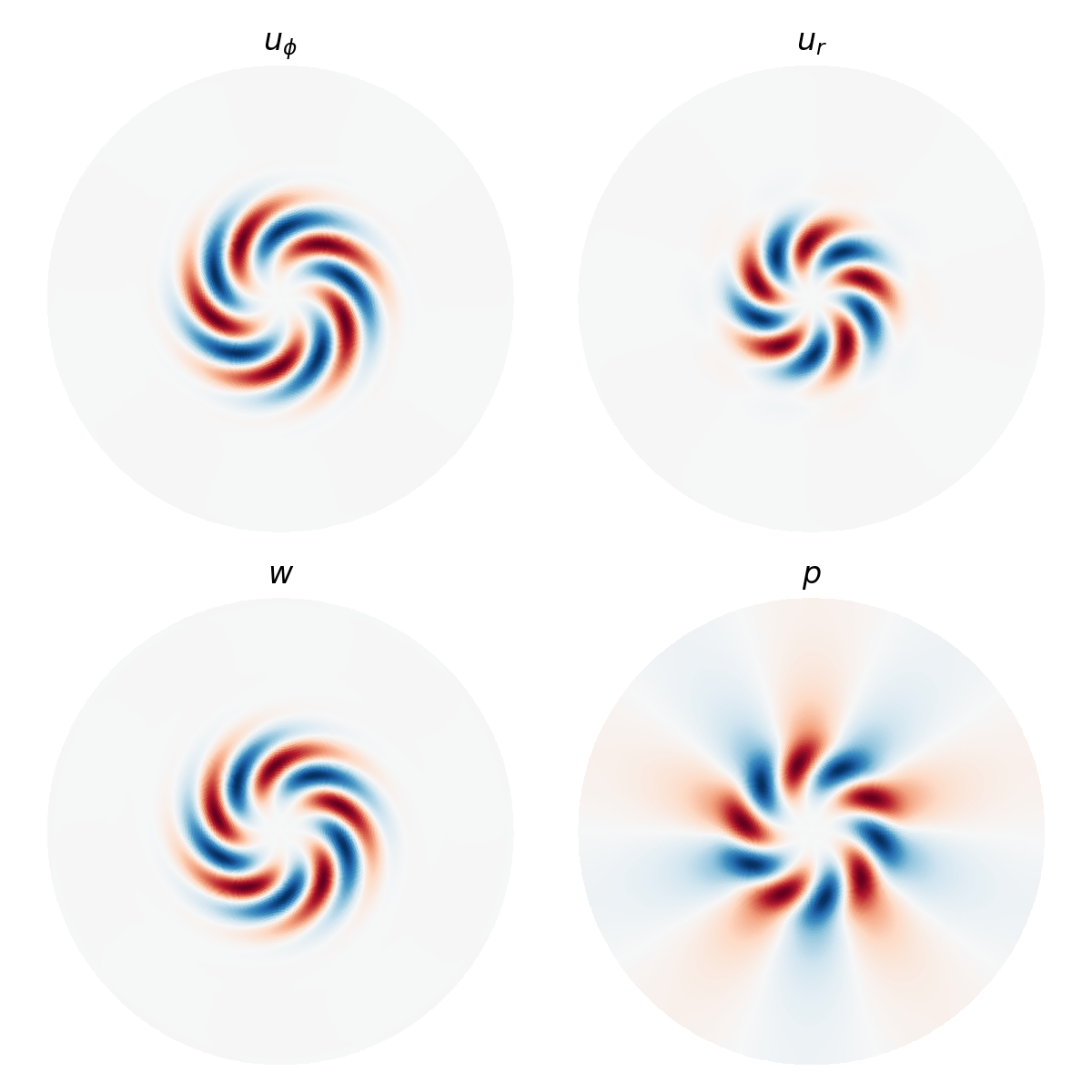
# Plot eigenfunction
scales = (32, 4)
ω = d3.div(d3.skew(u)).evaluate()
ω.change_scales(scales)
u.change_scales(scales)
w.change_scales(scales)
p.change_scales(scales)
phi, r = dist.local_grids(disk, scales=scales)
x, y = coords.cartesian(phi, r)
cmap = 'RdBu_r'
fig, ax = plt.subplots(2, 2, figsize=(6, 6))
ax[0,0].pcolormesh(x, y, u['g'][0].real, cmap=cmap)
ax[0,0].set_title(r"$u_\phi$")
ax[0,1].pcolormesh(x, y, u['g'][1].real, cmap=cmap)
ax[0,1].set_title(r"$u_r$")
ax[1,0].pcolormesh(x, y, w['g'].real, cmap=cmap)
ax[1,0].set_title(r"$w$")
ax[1,1].pcolormesh(x, y, p['g'].real, cmap=cmap)
ax[1,1].set_title(r"$p$")
for axi in ax.flatten():
axi.set_aspect('equal')
axi.set_axis_off()
fig.tight_layout()
fig.savefig("pipe_eigenfunctions.png", dpi=200)